
Key components along the X-ray path before the sample position (40 m from the X-ray source IU24). From upstream, there are millisecond-shutter (MS shutter) and 1st set of X-ray beam position and intensity monitor (XBPM) called Rigi, sitting on the granite chopper stage (to accommodate a future chopper system for time-resolved measurements). These are followed by an attenuator, 1st set of JJ-slit-pinhole (JJ-SP1), 2nd set of XBPM (Civi), and 2nd set of JJ-slit-pinhole (JJ-SP2) sitting on the collimation granite stage. A motorized pindiode (5-mm dia. active area) situated 1 mm after the S3N4 vacuum-exit window can be moved into the beam path for centering the JJ-SP.


(a) Schematic diagram of the TPS 13A online two-column SEC-SWAXS/UV-Vis/MALS/DLS/RI system, based on an Agilent 1260 HPLC sample purification system. An autosampler injects the samples into the system. Path A leads the sample to a SEC column, whereas Path B bypasses the column. After the HPLC UV-Vis absorption detection, the sample flows into a quartz capillary cell for simultaneous UV-Vis absorption and SWAXS measurements on the same sample spot. The elution continues to an optional multi-angle-laser-light scattering (MALS) and dynamic light scattering (DLS) measurements, then default refractive index (RI) detection before fraction sample collection. (b) A close-up picture of the quartz capillary housing, with the pathways of the sample, camera, UV-vis light, and air and water cooling indicated. The X-ray beam is indicated by a red arrow.
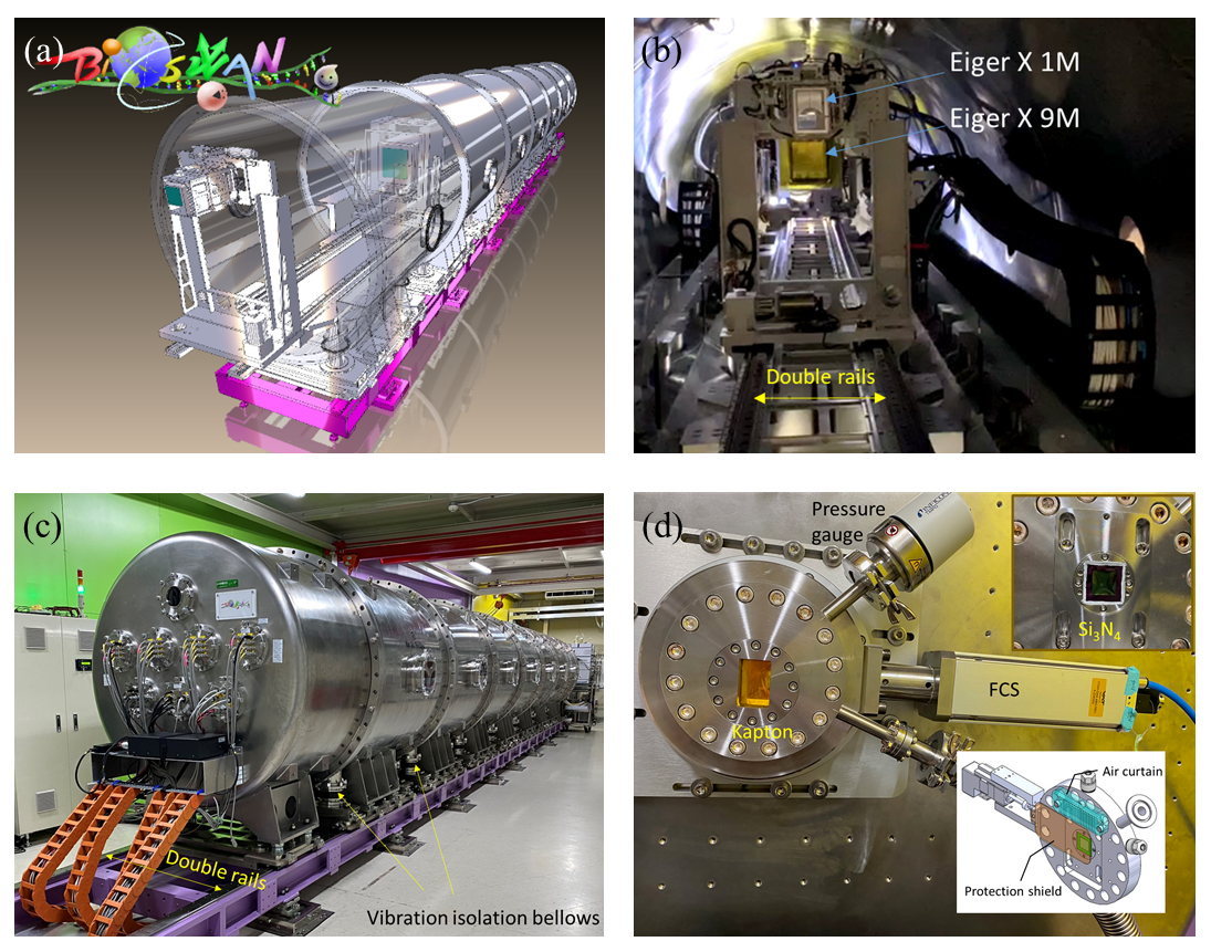
(a) Cartoon illustration of the vacuum vessel for the SWAXS detecting system at the TPS 13A endstation. (b) Inside the vacuum vessel, the Eiger X 1M (WAXS detector) sits on its stage, rolling on the rail system at the front; the Eiger X 9M (SAXS detector) is farther on the same rail system. (c) A back view of the detector vessel, with all the vacuum feedthroughs on the end tank. The detector vessel sits on another double-rail system to translate the whole system along the X-ray beam. Vibration isolation bellows (indicated) are installed to reduce the effects of detector vessel deformation during vacuum pumping on the precision rail alignment of the detector double-rail system enclosed inside the vacuum vessel. (d) Photograph of the entrance window and fast closing shutter (FCS) sealed with a Kapton window (40 mm by 60 mm) or a Si3N4 window (15 mm by 15 mm; upper right inset). The lower right inset shows a protection shield for the entrance window and an air curtain to be installed.
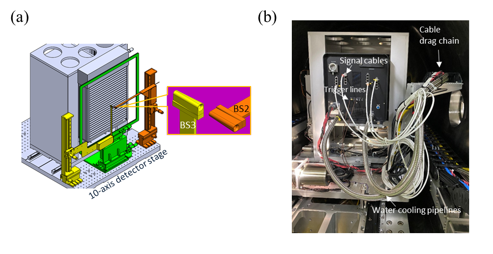
(a) Schematic diagram of the Eiger X 9M SAXS detector stage with 10 degrees of freedom as indicated by the 10 arrows, including ±120 mm detector translation in the vertical and horizontal directions. There is a house-made motorized aluminum roller to cover and protect the detector's active area when needed. A Ta beamstop (BS1) is glued on the center of a Kapton film of 8 µm thickness on the green frame (±20 mm in vertical and horizontal directions). The other two beamstops (BS2 and BS3, orange and yellow) are each equipped with a photodiode. (b) Back view of the Eiger X 9M, with all the signal and motor cables/air and water cooling lines carried by a cable drag chain as indicated.

(a) Illustration of the Eiger X 1M (E1M) with an opening of 35 mm by 60 mm. The beamstop BS4 (orange) is also shown on the detector stage of multi-degrees of freedom (tilt, rotation, horizontal movement, and vertical translation). Located at the right-bottom corner is a silicon drift detector (SDD, red circle) (b) Picture of the Eiger X 1M rotated by 90° from the orientation shown in (a). The cable drag chain that carries all relevant wirings is on the right.


(a) SEC-SWAXS data collection scheme mastered by the SEC system. Red path arrows represent trigger directions, and blue path arrows show the data flow. Data collection GUI (DC-GUI) is initiated by the sample system (SEC system in SEC-SWAXS), then executes a data collection plan through coordinating the X-ray detecting system with the other endstation components (e.g., Rigi/Civi XBPMs and ms-shutter). (b) DC-GUI for programmable data collection strategies up to 999 steps. For each step (row), users can set for either SAXS (SAS) or transmission mode (TM), the number of frames, wait time (between two frames), exposure time, hold time (before the next step), sample position, shifting of the predefined sample positions in horizontal or vertical directions, the attenuation factor of beam intensity (Att), sample temperature, and sample position rocking (to reduce radiation damage). Users can also choose which detector to use at the bottom-left corner. On the right-hand side, the millisecond shutter can be set to keep open during the whole data collection procedure or open only during the exposure time (to avoid unnecessary beam exposure to the sample).


(a) SAXS DR-GUI at TPS 13A, illustrated by a 10 mg/mL BSA sample solution with 100 µL injection. The upper part is used for transmission calculation, and the lower part is for the Eiger X 9M SAXS data reduction. Users input the sample file name, select detector image files, choose one of four image binning modes, and hit the Run button to conduct the reduction of the 2D images to the circularly averaged 1D I(q) profiles displayed at the lower right corner. Alternatively, line-cut profiles or region-of-interest (ROI) on a 2D pattern can be selected or rejected in the processing. (b) Parallel WAXS DR-GUI, operating independently or collectively (sharing the same instrument parameters) with the SAXS DR-GUI on the simultaneously measured SWAXS data. (c) The data evaluation page (DEP) with the SEC-SAXS data and online-UV absorption data measured at the same sample position over the sample elution. The DEP processes the data generated from SAXS DR-GUI to calculate SAXS I(0) (bottom left, red curve) and Rg (green curve) and display them with the sample concentration deduced from the online UV-Vis absorption (at a selected wavelength) for chromatographic evaluation (white curve). The upper right graph allows multi-profile comparison. The well-overlapped data profiles with similar Rg can be merged and converted into a p(r) function by clicking the yellow button. A DAMMIF simulation can then be selectively executed, with results displayed in the bottom right corner from an auto-preliminary data analysis.

Ethernet network of the TPS 13A endstation. The digital signals are communicated via the four Ethernet subnetworks: Science LAN (for data), EPCIS LAN (for beamline control), Galil LAN (for motors), and Device LAN (for others). All data are temporarily stored in a local NAS and updated to the DiCOS BioSAXS platform constructed by the Academia Sinica Grid Computing Centre (up-left corner) for storage, retrieval, and processing.
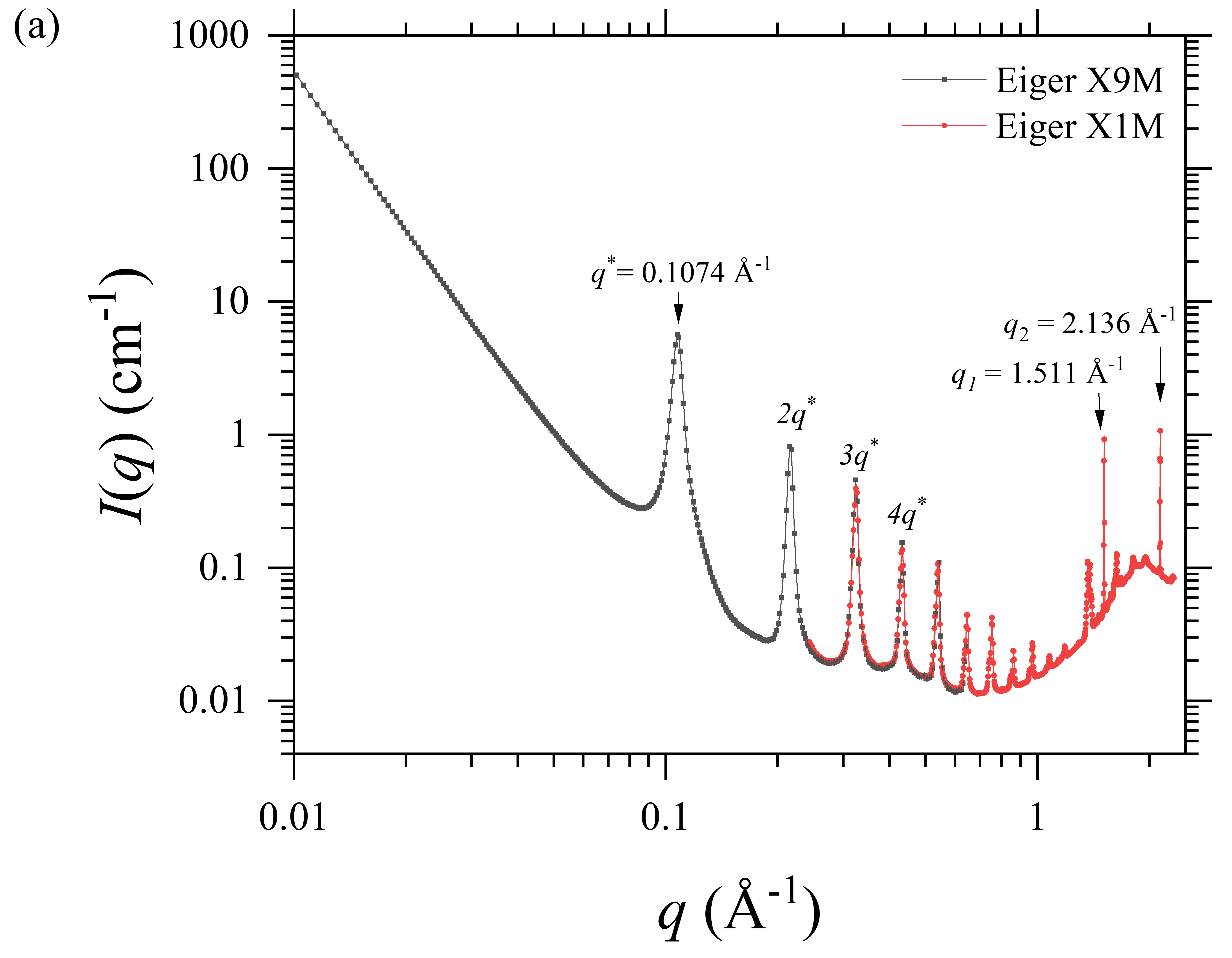
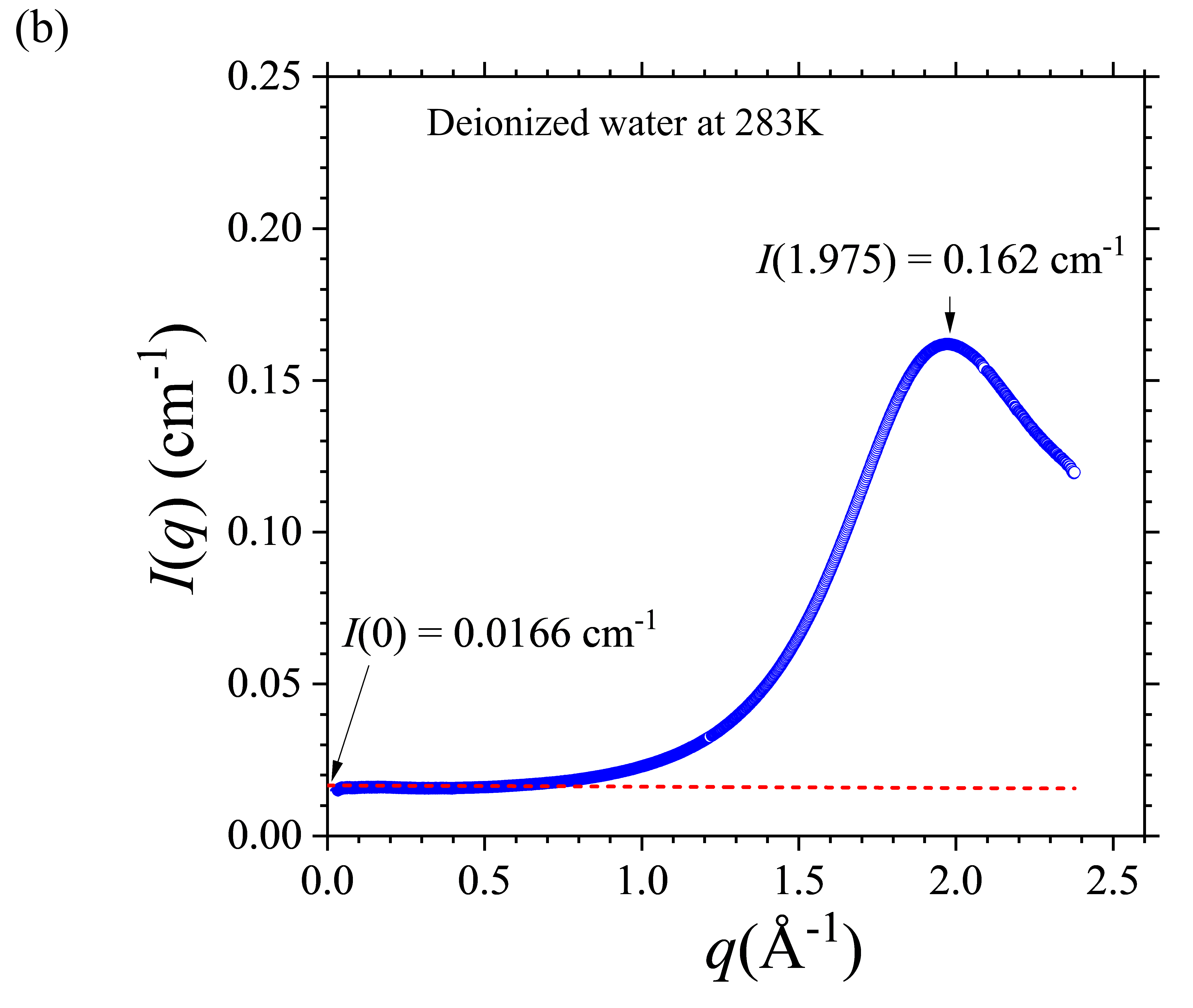
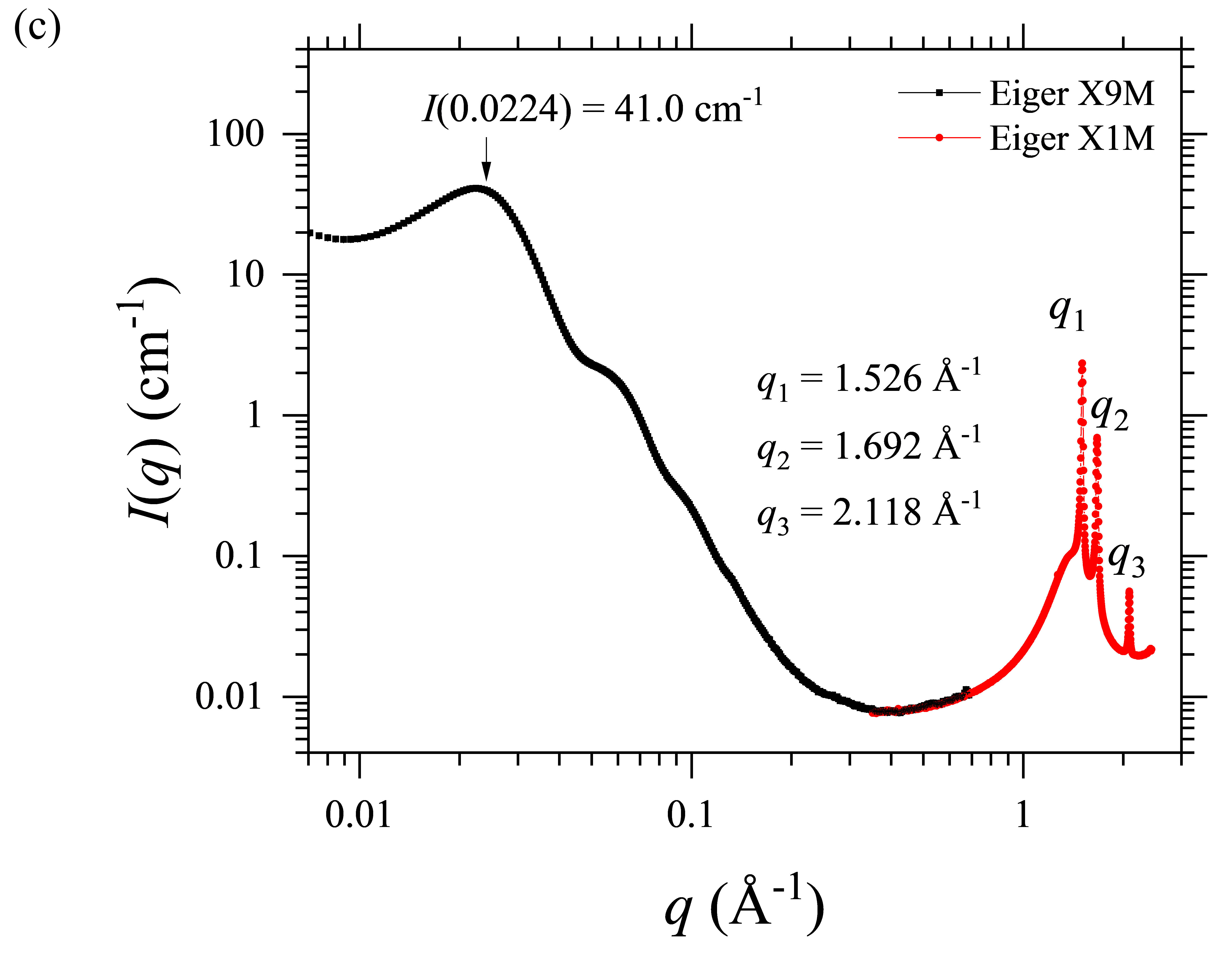
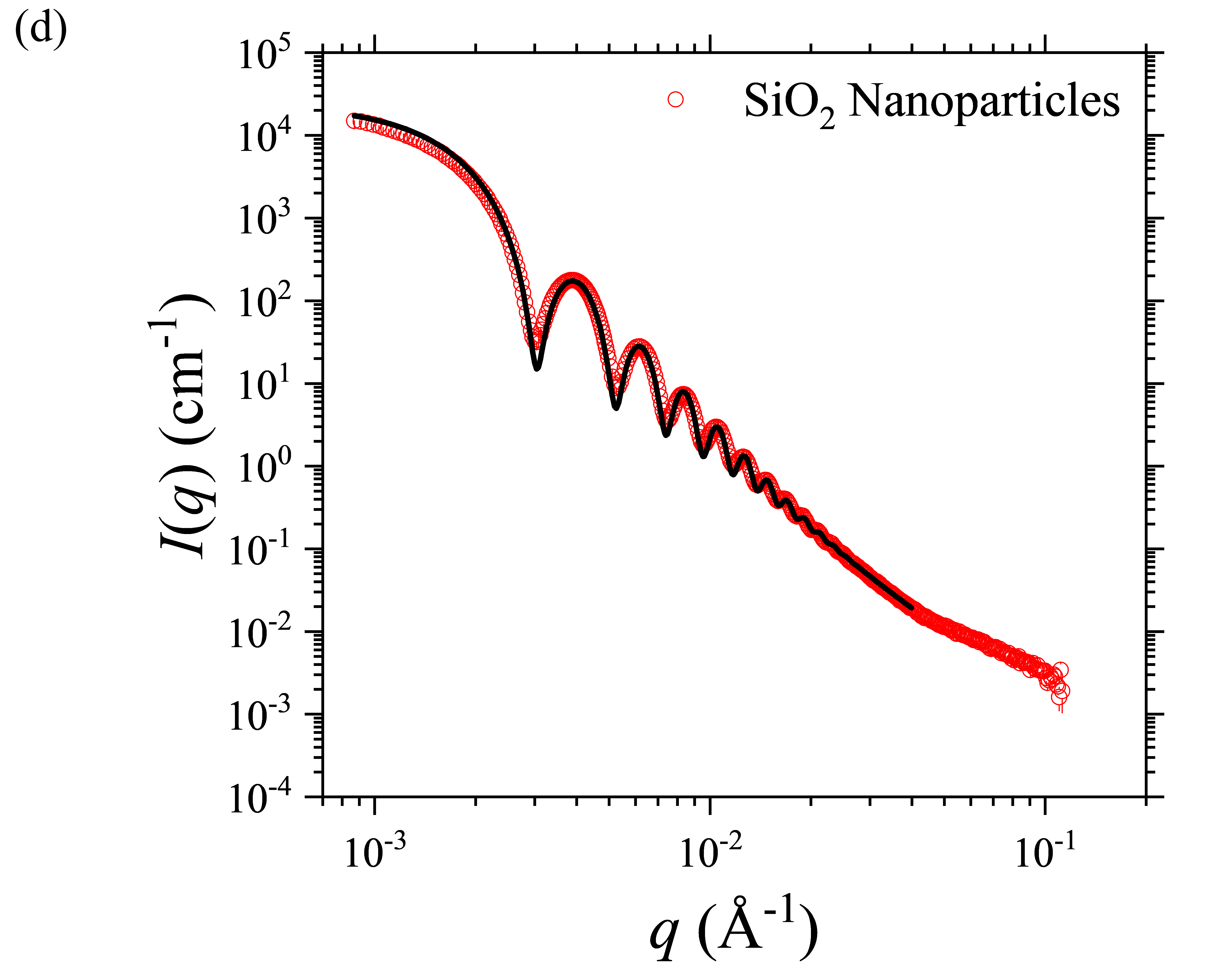
(a) Standard calibration of the SWAXS q value of the TPS 13A endstation using mixed powders of silver behenate (periodic peaks marked) and LaB6 standards (two characteristic peaks q1 and q2 indicated). An alignment factor is determined via scaling the SAXS data taken by Eiger X 9M and the WAXS data taken by Eiger X 1M. The factor is applied to all the subsequent SWAXS measurements. (b) SWAXS data of de-ionized water. The profile is scaled (with a scaling factor f) to reach an extrapolated (dotted line) I(0) value at 283 K, as indicated. The broad WAXS peak at ca. 1.975 Å-1 corresponds to a water correlation length. (c) SWAXS data measured for high-density polyethylene. It is calibrated by the standard procedure of water scattering and can serve as a secondary standard for q-position and absolute intensity using the calibrated values indicated. (d) USAXS data of SiO2 particles in solution, using a 10 keV beam and SD = 10.0 m. The data are fitted (solid curve) with 5% polydisperse core-shell spheres with a mean core diameter of 284 ± 11 nm and a shell thickness of 3.6 nm (with a slightly lower scattering length density than the core).
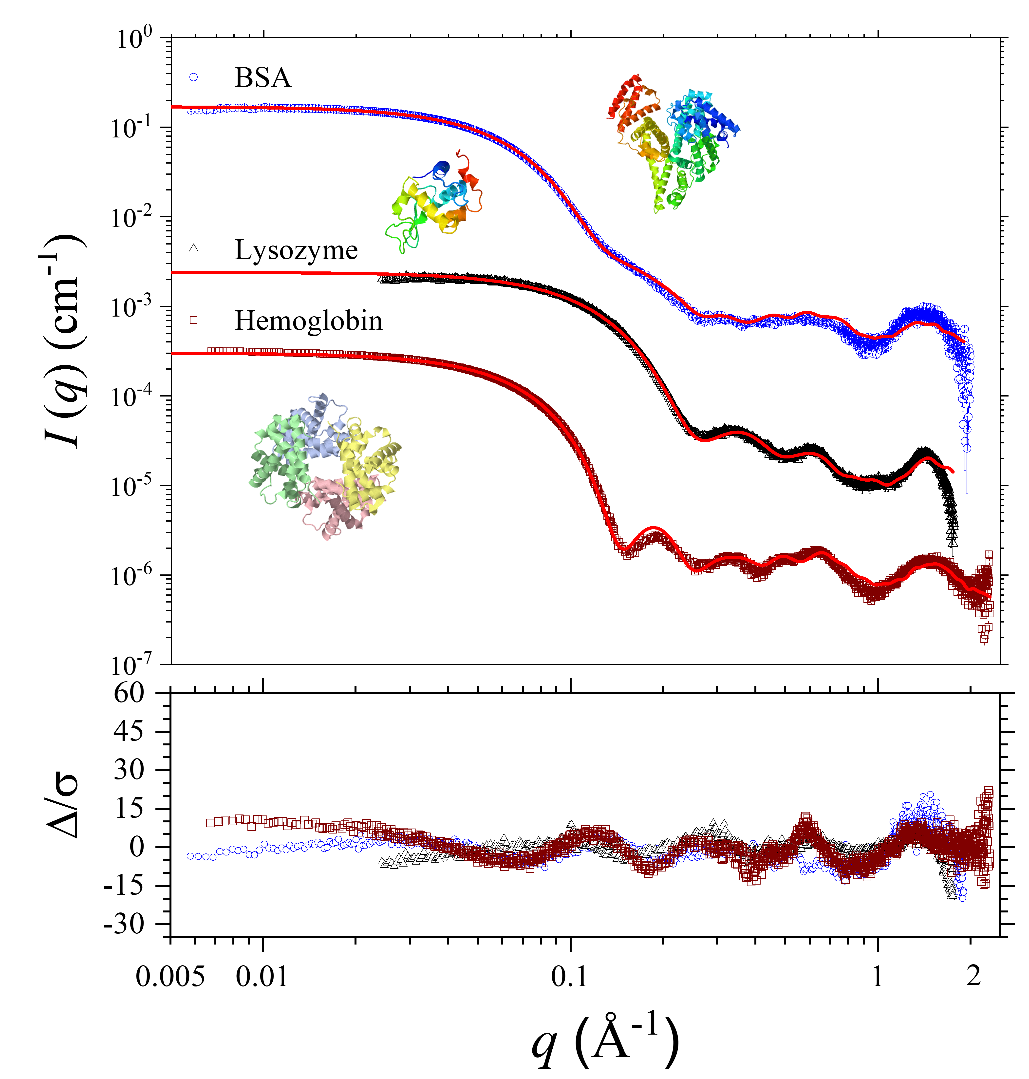
SWAXS data measured at TPS 13A for BSA (top), lysozyme (middle), and hemoglobin (bottom); also shown are the corresponding crystal structures. The sample concentrations are all 10 mg/mL. With 100 µL injection volume, the peak sample concentration during the HPLC elution reduces to ca. 4 mg/mL (cf. the dilution factors shown in Fig. S6). The WAXS data of BSA (Fig. S7) are replaced by that measured with the bypass mode (of little sample elution dilution effect) for better statistics. The lysozyme and hemoglobin intensity profiles are scaled down from the absolute intensity scales by 50 and 500. Also shown are the fitting curves calculated using CRYSOL (dotted red curves) based on the crystal structures with PDB ID 3V03 for BSA, 1LYZ for lysozyme, and 1A3N for hemoglobin. The lower inset shows the fitting residual D/s defined by the differences (D) of the model and experimental results normalized by the corresponding data uncertainties or errors s (Trewhella et al., 2017).
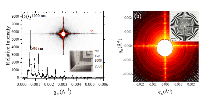
(a) USAXS pattern (inset) of an ensemble of gold L-shaped arrays of 2000-, 1000-, 500-, and 200-nm d-spacing (inset), measured using a 6-keV beam of DCM with 4BCC. The line-cut profile taken along the z-axis reveals the primary peak of the array of 1000-nm spacing located at q = 6.3x10⁻⁴ Å-1. The minimum detectable q is ca. 4.0´10-4 Å-1. (b) A USAXS data of a Siemens star pattern (inset), having 25-nm lines and space at the center zone. Note that the fine scattering features are differentiable down to q ~ 6x10⁻⁴ Å-1.
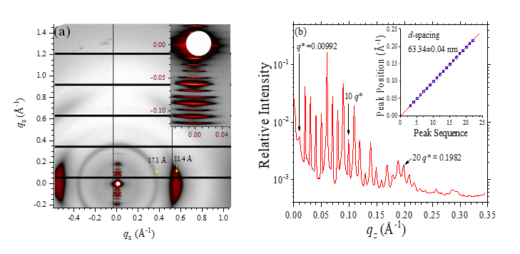
(a) Highly oriented 2D pattern taken from a turkey tendon, covering a wide q-range as indicated. Inset enlarges the details of the SAXS region for the periodic peaks along the qz direction. An associated arc along the qx axis is marked (yellow arrow) with the corresponding lateral dL-spacing of 11.4 Å. (b) The intensity line-cut profile extracted along the qz axis, with the periodic peaks selectively numbered. Inset shows that all the peak positions fall nearly perfectly on the linear regression line for the d-spacing indicated.

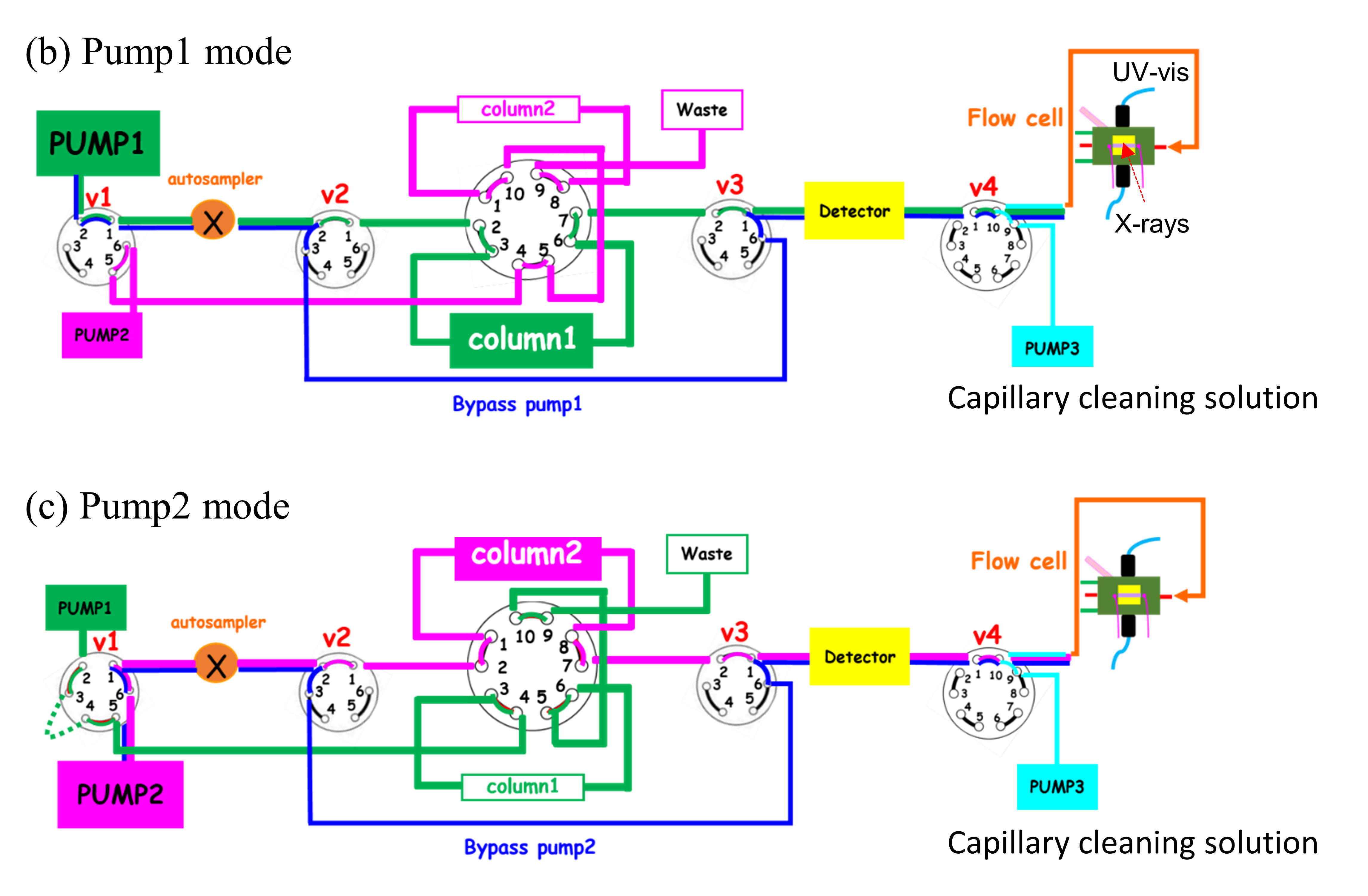
(a) Upper-half shows the VOYAGER™ GUI (under the VISION software hub of WYATT Technology Co.) used at the TPS 13A BioSWAXS beamline that integrates the Agilent 1260 HPLC operation and data collections of the UV-vis absorption, refractive index, multi-angle laser light scattering (MALLS), and dynamic light scattering (DLS); lower-half shows the data analyzed by the ASTRA GUI of VISION. (b) HPLC pump1 mode with column1 in duty while column2 in cleaning, and (c) Pump2 mode with column2 in duty, while column1 in cleaning. Either pump1 or pump2 can drive the bypass path (blue lines). The three pumps (pump1-3), four 6-way valves (v1-v4), and one 10-way valve (at the center) are marked. The capillary cell cleaning path is shown to the right-hand side with pump3. An online sample-mixing mode is also available.

The SAXS profiles of the sample capillary at the TPS 13A endstation collected before, during, and after a standard washing sequence. The results illustrate different stages and degrees of residual/damaged protein deposition on the sample capillary, including (1) right after sample data collection (black), (2) after 2 min of buffer flowing (red), and (3) adding 3 min of Hellmanex™ III flow followed by 3 min of DIW flow. After one washing sequence, the capillary shows no trace of protein deposition.
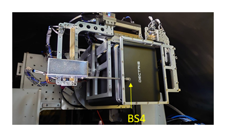
Motorized BS4 of Eiger 1M detector on the detector stage. BS4 is equipped with a photodiode and can translate for ±50 mm in vertical and horizontal directions.
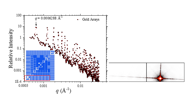
USAXS profile of a standard pattern of gold arrays (inset) extracted from the 2D pattern (on the right-hand side) measured using a 6 keV beam and a sample-to-detector distance of 10.0 m. The arrow marks the first SAXS peak at q = 0.0006288 Å-1, corresponding to the 1.0 µm pattern (red square in the inset). The peak width (~0.00004 Å‑1) reveals the q-resolution of the USAXS mode at the peak position.